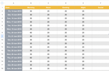
I'm making a spreadsheet in numbers to track the time carers spend looking after someone each day. I've got the date in the first column and the times after that. I wanted an easy way to tell the weeks apart, like a dotted line border on the cells at the end of each week, but I just can't figure it out how to do it. See the screenshot attached. Thanks.
Got a tip for us?
Let us know
Become a MacRumors Supporter for $50/year with no ads, ability to filter front page stories, and private forums.
Border at the end of each week in Numbers
- Thread starter libdom
- Start date
- Sort by reaction score